Hello blog readers!

Here is another tl;dr; blog post! Yesterday I completed my winter exam session at university and want to recall one interesting work I had year ago at the course called “Data structures and algorithms” where we learned various data structures and manipulation algorithms. During the course we developed them in programming languages with further analysis. In array search class work I had to implement, analyze and compare two search methods: sentinel search and hash table search.

Most search algorithms have complexity. This means that their performance depends on array size. Larger is array, more time is required to find element in array. There is binary search that gives which better than linear, but still depends on array size and requires sorted array. Binary search is impossible for unsorted arrays. What next? Next is search algorithm that would give us constant complexity. This means that regardless of array size, search will be completed in constant time. This algorithm (actually, data structure) is hash table.

What is hash table? It is an associative array that maps keys to data values. Unlike classic arrays, there is no such term as array index, instead there used term key value. Key is an identification information about data value. During class work I learned a lot about hash tables and faced a number of very interesting challenges while attempting to develop a reliable implementation of hash table. And this blog post will reveal all of them!

Hash functions

Prior to talking about hash tables we need to explain how keys are derived. Keys are derived from data value by passing them through some hash function. Hash function is a function that accepts data of arbitrary size and returns integral value of fixed size which is usually less than input size. All hash functions share the same common properties:

• Codomain of hash function less or equal to , where — is return value’s size in bits.
• Hash value has no “memory”, i.e. you cannot restore original data from hash value.
• By passing the same data to the same function multiple times, result is identical.

Hash function’s return value is called hash code. It is the same what you do when calculating cryptographic hashes (you are probably familiar with). You can take a 10GB file and compute an SHA1 hash. You will receive a 20-byte fixed-size value that uniquely (with some exceptions) identifies the file contents. If you take a 5 byte file, SHA1 hash will still be 20 bytes long. Hash code value for a given hash algorithm is always of fixed size. Here we get why hash table is associative array: you associate keys with data (values).

When implementing hash table, keys are used as hints to determine where the data value is actually stored in memory, so you can find data value in hash table with a constant find time of , whether hash table size is 5 or 5 millions items. Actually, we do not care about exact hash function’s implementation to produce hash codes, it can be any as long as key can identify the data it is associated with.

Challenge 1 — Internal structure

Ok, we have keys and data values. How would we store data value in hash table internally? The most evident way is to use classic linear array. Next, we need to determine what we will store. We will store keys and data values associated with keys. Both in the same slot in internal array. So, we introduce new term: bucket. Bucket is a structure with two fields to store key value and data value. Although, key value storage in hash table may not be evident right now, it plays important role in hash table’s slot management. Internal array we will call as bucket array.

Bucket position in this array depends on two factors: key value and bucket array size. So, we take key, bucket array size and pass it through another function with two arguments: , where is key value and is bucket array size. The result of this hash function will be actual index in bucket array. We cannot use key values directly to denote bucket array’s index, because key value generation function is independent from hash table implementation and can be fairly large. For example, if we use SHA1 hashes as keys, internal array’s size would be , where s is bucket size in bytes. Therefore we need another hash function. At this point we can define two hashing functions:

1. Hashing function is used to produce a compressed digest computed over data value. Result value is data value’s hash code. Its size is fixed for a given hashing function.
2. Hashing function to produce a compressed digest computed over key value and internal array’s size. Result value is the index in internal array to store value. Obviously, result value is in range from 0 to bucket array’s size. Upper bound limit is easily accomplishing by using division with remainder math operation. So, any hash function will have the following scheme: where is bucket array size. We take modulus against function to ensure that value is always positive.

Observation of hash function’s argument list leads us to another important conclusion: if we change bucket array size, we have to re-hash entire table, because second parameter of the function is changed and for the same key value will return different bucket index value. In order to maintain hash table consistency, we create new bucket array with new size. Take one by one buckets from original bucket array, pass them through the same function (with new l parameter) and destroy original bucket array when all items are repositioned in resized array. This gives us serious performance hit. As the result, it is strongly recommended to create hash table with a size enough to store all buckets in advance in order to avoid re-hash operations.

Challenge 2 — Hash function collisions

So far so good. Further analysis gives us another fundamental issue we have to care about. Since hash value is of fixed size and usually less than data value size, hash function will lead to collisions. Hash collision occurs when two distinct inputs produce the same output. What does it mean in hash table terms? This means that when attempting to insert another distinct key it will pretend to slot that is already occupied by another key:

 

Keys are different, but index in bucket array is the same and we should handle this somehow. There are several approaches, the most popular are:

• Linear probing

With linear probing you are increasing index by one until free slot is found:

Here we see a hash table with 10 slots and filled 4 slots. When attempting to insert number 52, it pretends to slot 2. This slot is already occupied, so we increase slot index until we find empty slot and put value there. Although, very easy, it is very inefficient when there are many sequentially occupied slots. As more elements hash table contains, more time is spent to find free slot to insert the bucket.

• Bucket chaining

With bucket chaining, bucket array is represented as a 2-dimensional array where each slot is an array to store buckets with matching slot index:

This approach is more effective than linear probing, because we don’t have to search empty slot to insert the bucket. However, when searching the array, chaining approach takes linear time to find the right bucket in embedded array, because it is linear. Therefore, chaining approach is efficient when inserting buckets to hash table, but is less efficient when searching bucket.

• Open addressing

In open addressing we apply different hash function to get new insert slot index:

Different functions will produce different slot index for the same key. If new slot is still occupied, apply different hashing functions until empty slot is found. Doesn’t sound promising. And open addressing complicates search functions, because you have to apply the same set of hash functions in exact order to find the requested bucket or report that bucket is not found. We report “element not found” error when hash function returns empty slot during search.

Challenge 3 — Hash table deletion anomalies

We solved one problem and the next issue is already here. It occurs immediately when we implement bucket deletion functionality. This will immediately break linear probing and open addressing collision resolution mechanisms. Here is why.

• Linear probing deletion anomaly

When searching with linear probing, we attempt to find the requested bucket at the first slot index calculated by hash function. If the slot is not empty, increase slot index by one until we find requested bucket, or report “element not found” error when hitting empty slot. In a given example, we successfully found requested bucket in 5 steps. Now, remove bucket at slot 4:

Although, the bucket 52 is stored in hash table at slot 6, we hit empty slot at slot 4. By convention, we have to return “element not found” error. An attempt to continue probing to the end of bucket array will kill the whole purpose of hash table and searching will take time.

• Open addressing deletion anomaly

Normally, we will apply a set of different hash functions in exact order used during bucket insertion until we find requested bucket or hit empty slot. If we reached empty slot, report “element not found” error. Now, remove bucket at slot 4:

Once again, by convention, we have to report “element not found” if we hit empty slot during bucket search. Requested bucket is stored in hash table, but we can’t reach it due to deletion anomalies.

In order to solve deletion anomalies we have to modify bucket deletion by adding new step and marking deleted slot as deleted. Simple flag that there once was bucket, it no longer stored. And modify search algorithm to treat “deleted” flag as occupied. And here is how the whole thing would work:

• “Deleted” flag is transparent for insertion operations. When inserting new bucket, “deleted” flag is ignored and can be overwritten by new bucket.
• “Deleted” flag is respected by search operations and treated as occupied.

by using this behavior we effectively eliminate bucket deletion anomalies:

The only downside of this solution is that comparison number at each step increased by one. During each loop iteration we have to check :

• Current slot value matches requested key. Outcome: return bucket.
• Current slot contains “deleted” flag. Outcome: continue loop.
• Current slot is empty. Outcome: return “element not found”.

Here we can make another important conclusion: bucket array size must be larger than hash table capacity for at least 1 element. This means that when hash table is full, there is at least one empty slot in bucket array. It is necessary to have it in order to determine that requested key was not found. Otherwise, we will end up in an infinity loop when requested key is not stored in hash table. As the result, we have to check if hash table public capacity (visible to clients) is always less than bucket array size (hidden from clients).

Implementing Open Addressing collision resolution mechanism

For my class work I selected Open Addressing collision resolution mechanism as more challenging. And it really was.

• Challenge 4 — consistent set of functions used during insertion and search operations when collision occurs

How would I keep an ordered list (of variable length) of distinct hash functions without remembering them in memory? The obvious way is to use base function and put multiplicative factor inside. For example, base function is: where is bucket key value and is bucket array size. Introduce multiplicative factor: . Multiplicative factor may have value: . Quick function test confirms serious problem when key value and bucket array size share the same common divisor. Suppose, bucket array size is 10:

PS C:\> PS C:\> 1..10 | %{($_ * 7) % 10}
7
4
1
8
5
2
9
6
3
0
PS C:\> 1..10 | %{($_ * 5) % 10}
5
0
5
0
5
0
5
0
5
0
PS C:\> 1..10 | %{($_ * 4) % 10}
4
8
2
6
0
4
8
2
6
0
PS C:\>

In the first example, key value is 7. 7 and 10 do not share common divisors, therefore applying hash function against key value multiple times (literally, up to times), slot indexes are always distinct. However, key values 5 and 4 share common divisors with 10 (bucket array size): 5 and 2 respectively, as the result, function falls in to cycles and may never find empty slot index, because not all slot indexes are checked.

• Challenge 5 — eliminate cycles during slot index calculation

Provided example observation suggests that bucket array size must not share common factor with key value. The most reliable way to accomplish this is to align bucket array size to smallest prime number that is larger than public hash table size + 1. A prime number is a natural number greater than 1 that has no positive divisors other than 1 and itself. “+1” is necessary to provide extra empty slot if public hash table size is already prime number. In this case, we have to find another prime number. Therefore, when client define hash table public size, we have to resize bucket array to nearest prime value.

Challenge 6 — find and test prime number

As I stated above, prime number is a natural number greater than 1 that has no positive divisors other than 1 and itself. In order to test whether the number is prime it would be necessary to attempt to divide with remainder all numbers that are less then candidate. For large numbers that would result in huge number of division trials. If prime candidate is non-prime it will have at least one common divisor that is in range where is common divisor and is prime number candidate. More details on wikipedia. I’m using trial division approach to determine whether the particular number is prime or not:

static Boolean isPrime(Int32 number) {
    Int32 boundary = (Int32)Math.Floor(Math.Sqrt(number));
    if (number == 1) { return false; }
    if (number == 2) { return true; }
    for (Int32 i = 3; i <= boundary; i += 2) {
        if (number % i == 0) { return false; }
    }
    return true;
}

Ok, we know how to determine whether the number is prime or not. I was wondering how much values I have to test in order to find smallest prime that is larger than bucket size array? I calculated distance between each neighbor primes in range from 3 to 1 000 000:

This diagram (generated by R) tells us that common distance between neighbor primes lies in range from 1 to 20-25, while absolute average distance is 12.73. Therefore, in order to find required prime we will have to perform trial division test for about 6 (12/2) numbers in average.

Results

At this point I got a decent hashing function, collision and deletion anomaly resolution algorithms. Now we are going to test final solution. I made 4 tests:

• Test 1 — bucket array size as small as possible
• Test 2 — bucket array size is +10% than hash table public size
• Test 3 — bucket array size is +20% than hash table public size
• Test 4 — bucket array size is +30% than hash table public size

Each test includes 10 key search trials for each of 10 different hash table sizes. Hash table is filled with random numbers. First trial for each hash table size was made when searching non-existent key. Actual collision count during each iteration is: (Number of comparisons – 1) / 2.

Test 1

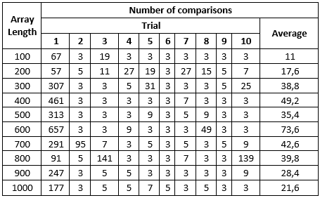
This table shows us an unacceptable large count of collisions occurred during non-existent key search and still relatively large number of collisions occurred during search for existent key. This means that small amount of empty space in bucket array make our hash table very inefficient.

Test 2

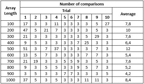
When increasing bucket array size by 10% comparing to hash table size, numbers become much-much better. Even worst non-existent key search resulted in just 25 collisions. Existent key search in many cases completed from a first attempt.

Test 3

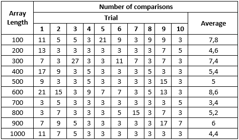
When increasing bucket array size by 20% comparing to hash table size, numbers become slightly better. Not that dramatically, but way better. Worst search trial resulted in just 10 collisions.

Test 4

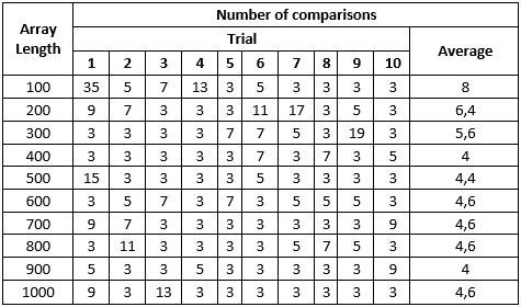
When increasing bucket array size by 30% comparing to hash table size, numbers remain almost the same. As the result, we can conclude that in a given implementation of hash table, the most efficient configuration is when bucket array size is larger than hash table size by 20%. Further bucket array increase doesn’t give improvements and wastes memory for nothing.

Final chart

And here is final chart that summarizes all results:

Downloads

Here is my final Visual Studio project that implements sentinel and hash table search engines:

---